中性子の基本的性質

熱・冷中性子を対象とした中性子実験でよく使う計算をまとめる。

はじめに基本定数をまとめておく。

from math import pow, sqrt, pi, exp
from scipy import constants as phys
import sympy
import handcalcs.render

%%render sci_not 2
#Parameters
e = phys.e # c
c = phys.c # m/s
m_n = phys.m_n*phys.c**2/phys.e # eV
h = phys.h/phys.e  #  $\rm eV \cdot s$
hbar = phys.h/phys.e/2/phys.pi # $\rm eV \cdot s$
k_B = phys.k # J/K
N_A = phys.N_A # $\rm /m^3$

\[ \begin{aligned} e &= 1.60 \times 10 ^ {-19} \; \;\textrm{(c)} &c &= 3.00 \times 10 ^ {8} \; \;\textrm{(m/s)} &m_{n} &= 9.40 \times 10 ^ {8} \; \;\textrm{(eV)} \\ h &= 4.14 \times 10 ^ {-15} \; \;\textrm{($\rm eV \cdot s$)} &\mathrm{hbar} &= 6.58 \times 10 ^ {-16} \; \;\textrm{($\rm eV \cdot s$)} &k_{B} &= 1.38 \times 10 ^ {-23} \; \;\textrm{(J/K)} \\ N_{A} &= 6.02 \times 10 ^ {23} \; \;\textrm{($\rm /m^3$)} \end{aligned} \]

波長、エネルギー、温度、速度の換算

ある運動エネルギー \(E\) を持った中性子は \[ E = \frac{\hbar^2 k^2}{2m} = \frac{h^2}{2m\lambda^2} = \frac{1}{2}mv^2 = k_BT \] で書けるから、ある波長\(\lambda\)の時のエネルギーと温度は

%%render sci_not 2
lambda_ = 0.18*1e-9 # m
E = h**2/(2.*(m_n/c**2)*lambda_**2)*1e3 #meV
T = E*1e-3/(k_B/e) #K

\[ \begin{aligned} \mathrm{lambda}_{} &= 0.18 \cdot 1 \times 10 ^ {-9} &= 1.80 \times 10 ^ {-10} \; \;\textrm{(m)} \\ E &= \frac{ \left( h \right) ^{ 2 } }{ 2. \cdot \left( \frac{ m_{n} }{ \left( c \right) ^{ 2 } } \right) \cdot \left( \mathrm{lambda}_{} \right) ^{ 2 } } \cdot 1 \times 10 ^ {3} \\&= \frac{ \left( 4.14 \times 10 ^ {-15} \right) ^{ 2 } }{ 2. \cdot \left( \frac{ 9.40 \times 10 ^ {8} }{ \left( 3.00 \times 10 ^ {8} \right) ^{ 2 } } \right) \cdot \left( 1.80 \times 10 ^ {-10} \right) ^{ 2 } } \cdot 1 \times 10 ^ {3} \\&= 2.52 \times 10 ^ {1} \; \;\textrm{(meV)}\\ \\ T &= E \cdot \frac{ 1 \times 10 ^ {-3} }{ \frac{ k_{B} }{ e } } = 2.52 \times 10 ^ {1} \cdot \frac{ 1 \times 10 ^ {-3} }{ \frac{ 1.38 \times 10 ^ {-23} }{ 1.60 \times 10 ^ {-19} } } &= 2.93 \times 10 ^ {2} \; \;\textrm{(K)} \end{aligned} \]

ある波長の中性子の速度\(v\)は \[ \lambda = \frac{h}{mv} \] だから

sympy.init_printing()
sympy.var('lambda_, v')
sympy.Eq(lambda_, h/(m_n/c/c)*1e9/v)

\(\displaystyle \lambda_{} = \frac{395.603400611944}{v}\)

となる。

しれっと中性子エネルギーと温度の換算をしたが、実際のところ中性子の温度分布はボルツマン分布に従った幅のある分布を持っているため、温度とエネルギーは1対1で決めることはできない。 上記計算で求めた温度は平均値に相当する。

TOF法

パルス中性子源で用いられるtof(time of fright)と対応させるには、小学生の時習った時間・距離・速さの関係を使えばいいから

sympy.var('lambda_, TOF, L')
sympy.Eq(lambda_, (h/(m_n/c/c)*1e9 /L)*TOF)

\(\displaystyle \lambda_{} = \frac{395.603400611944 TOF}{L}\)

ちなみにこの395.6という数字、よく使うから覚えといた方がいいかもしれない。

数密度の計算

数密度は、密度\(\rho\), 原子量\(M\), アボガドロ数\(N_A\)を用いて \[ N = \frac{\rho}{M}N_A \] で書ける。　

Niの場合、

%%render sci_not 2
#Parameters
rho_Ni = 8.908 # $\rm g/{cm}^3$
M_Ni   = 58.6934 #g/mol
N_Ni   = rho_Ni*1e6/M_Ni*N_A # $\rm /m^3$

\[ \begin{aligned} \rho_{Ni} &= 8.91 \times 10 ^ {0} \; \;\textrm{($\rm g/{cm}^3$)} &M_{Ni} &= 5.87 \times 10 ^ {1} \; \;\textrm{(g/mol)} &N_{Ni} &= 9.14 \times 10 ^ {28} \; \;\textrm{($\rm /m^3$)} \\ \end{aligned} \]

有効ポテンシャルの計算

簡単な系

有効ポテンシャルは \[ U = \frac{2\pi\hbar^2}{m}bN \] であるから、

%%render sci_not 2
# Parameters
b_Ni = 10.3*1e-15 #m
U_Ni = (2*pi*hbar**2)/(m_n/c**2) * (b_Ni)*N_Ni #eV

\[ \begin{aligned} b_{Ni} &= 1.03 \times 10 ^ {-14} \; \;\textrm{(m)} &U_{Ni} &= 2.45 \times 10 ^ {-7} \; \;\textrm{(eV)} \end{aligned} \]

化合物の場合

化合物の場合、有効ポテンシャルは \[ U = \frac{2\pi\hbar^2}{m_n}\sum_i b_i N_i \]

と書ける。
つまり各元素の数密度がわかればいい。
化合物の数密度は、ある元素\(i\)の原子数\(M_i\)の物質の質量分率を\(R~\rm(wt\%)\)としたとき、 \[ N_i = \frac{\rho_\mathrm{tot}}{M_i}N_A\times R \] となる。

よって、有効ポテンシャルは \[ U = \frac{2\pi\hbar^2}{m_n}\rho_\mathrm{tot}N_A\sum_i \frac{b_iR_i}{M_i} \] で得られる。

組成式がわかっている場合は、質量分率を使わずに計算できる。 一般的な化合物 \(a_xb_yc_z\)の場合、原子量は \[ M_{\rm tot} = xM_a+yM_b+zM_c \] で得られる。 このとき、化合物の数密度は \[ N_{\rm tot} = \frac{\rho}{M_{\rm tot}}N_A \] であり、それぞれの元素に対しては \[ N_a=xN_{\rm tot},\quad N_b=yN_{\rm tot},\quad N_c=zN_{\rm tot} \] と書くことができる。 これより、 \[ U= \frac{2\pi\hbar^2}{m_n} N_{\rm tot}\left( xb_A+yb_B+zb_C \right) \] となる。

適当に\(\mathrm{SiO_2}\)の場合を考える

%%render sci_not 2
rho_SiO2 = 2.2 # $g/cm^3$
M_Si     = 28.0855 # g/mol
M_O      = 15.9994 # g/mol
M_SiO2   = 2*M_O + M_Si # g/mol
N_SiO2   = rho_SiO2/M_SiO2*N_A*1e6 # $\rm /m^3$

b_Si   = 4.1491e-15 # m
b_O    = 5.803e-15 # m
b_SiO2 = (b_Si*1 + b_O*2) # m
U_SiO2 = (2*pi*hbar**2)/(m_n/c**2) * b_SiO2 * N_SiO2  # eV

\[ \begin{aligned} \rho_{SiO2} &= 2.20 \times 10 ^ {0} \; \;\textrm{($g/cm^3$)} \\ M_{Si} &= 2.81 \times 10 ^ {1} \; \;\textrm{(g/mol)} \\ M_{O} &= 1.60 \times 10 ^ {1} \; \;\textrm{(g/mol)} \\ M_{SiO2} &= 2 \cdot M_{O} + M_{Si} = 2 \cdot 1.60 \times 10 ^ {1} + 2.81 \times 10 ^ {1} &= 6.01 \times 10 ^ {1} \; \;\textrm{(g/mol)} \\ N_{SiO2} &= \frac{ \rho_{SiO2} }{ M_{SiO2} } \cdot N_{A} \cdot 1 \times 10 ^ {6} = \frac{ 2.20 \times 10 ^ {0} }{ 6.01 \times 10 ^ {1} } \cdot 6.02 \times 10 ^ {23} \cdot 1 \times 10 ^ {6} &= 2.21 \times 10 ^ {28} \; \;\textrm{($\rm /m^3$)} \\ b_{Si} &= 4.15 \times 10 ^ {-15} \; \;\textrm{(m)} \\ b_{O} &= 5.80 \times 10 ^ {-15} \; \;\textrm{(m)} \\ b_{SiO2} &= 1.58 \times 10 ^ {-14} \; \;\textrm{(m)} \\ U_{SiO2} &= \frac{ 2 \cdot \pi \cdot \left( \mathrm{hbar} \right) ^{ 2 } }{ \frac{ m_{n} }{ \left( c \right) ^{ 2 } } } \cdot b_{SiO2} \cdot N_{SiO2} \\&= \frac{ 2 \cdot 3.14 \times 10 ^ {0} \cdot \left( 6.58 \times 10 ^ {-16} \right) ^{ 2 } }{ \frac{ 9.40 \times 10 ^ {8} }{ \left( 3.00 \times 10 ^ {8} \right) ^{ 2 } } } \cdot 1.58 \times 10 ^ {-14} \cdot 2.21 \times 10 ^ {28} \\&= 9.05 \times 10 ^ {-8} \; \;\textrm{(eV)}\\ \end{aligned} \]

屈折率

中性子に対する物質の屈折率\(n\)は \[ n = \sqrt{1 - \frac{U}{E}} \] で書ける、\(U\)は上記で求めた有効ポテンシャルを入れれば良い。

%%render sci_not 2
E = 0.025 #eV
delta_n = 1 - sqrt(1 - U_SiO2/E) 

\[ \begin{aligned} E &= 2.50 \times 10 ^ {-2} \; \;\textrm{(eV)} \\ \delta_{n} &= 1 - \sqrt { 1 - \frac{ U_{SiO2} }{ E } } = 1 - \sqrt { 1 - \frac{ 9.05 \times 10 ^ {-8} }{ 2.50 \times 10 ^ {-2} } } &= 1.81 \times 10 ^ {-6} \end{aligned} \]

波長を用いて書き直すと

%%render sci_not 5
U = U_SiO2 #eV 
h #eV*s
m_n # eV
lambda_ = 1e-9 #m
n = sqrt(1-U/(h**2/2/(m_n/c/c)/lambda_**2))

\[ \begin{aligned} U &= 9.04606 \times 10 ^ {-8} \; \;\textrm{(eV)} \\ h &= 4.13567 \times 10 ^ {-15} \; \;\textrm{(eV*s)} \\ m_{n} &= 9.39565 \times 10 ^ {8} \; \;\textrm{(eV)} \\ \mathrm{lambda}_{} &= 1.00000 \times 10 ^ {-9} \; \;\textrm{(m)} \\ n &= \sqrt { 1 - \frac{ U }{ \frac{ \left( h \right) ^{ 2 } }{ 2 } \cdot \frac{1} { \frac{ m_{n} }{ c } \cdot \frac{1} { c } } \cdot \frac{1} { \left( \mathrm{lambda}_{} \right) ^{ 2 } } } } \\&= \sqrt { 1 - \frac{ 9.04606 \times 10 ^ {-8} }{ \frac{ \left( 4.13567 \times 10 ^ {-15} \right) ^{ 2 } }{ 2 } \cdot \frac{1} { \frac{ 9.39565 \times 10 ^ {8} }{ 2.99792 \times 10 ^ {8} } \cdot \frac{1} { 2.99792 \times 10 ^ {8} } } \cdot \frac{1} { \left( 1.00000 \times 10 ^ {-9} \right) ^{ 2 } } } } \\&= 9.99945 \times 10 ^ {-1} \\ \end{aligned} \]

屈折率はほとんど1に近い値を取るため、しばしば以下の近似が用いられる。 \[ \sqrt{1+x} \simeq 1+\frac{x}{2} \] であるから、 \[ n \simeq 1 - \frac{V}{2E} = 1 - \frac{b_c N \lambda^2}{2\pi} = 1 - \frac{m U_\mathrm{Fermi} \lambda^2}{h^2} \] と書ける。

反射臨界角

中性子は有効ポテンシャルによって光学的な反射を行う。

その反射角は \[ \theta_c = \sqrt{\frac{bN}{\pi}}\lambda \] Niの場合、\(\theta_c\)は

%%render sci_not 2
# Parameter 
b_Ni = 10.3e-15 #m
#N_Ni #n/m^3
lambda_ = 1*1e-9 #m
theta_c = sqrt(b_Ni*N_Ni/pi)*lambda_ # rad/nm

\[ \begin{aligned} b_{Ni} &= 1.03 \times 10 ^ {-14} \; \;\textrm{(m)} &\mathrm{lambda}_{} &= 1.00 \times 10 ^ {-9} \; \;\textrm{(m)} &\theta_{c} &= 1.73 \times 10 ^ {-2} \; \;\textrm{(rad/nm)} \\ \end{aligned} \]

また、この時\(0.5~\rm eV\)中性子の反射臨界角は

%%render sci_not 2
E = 0.5 #eV
lambda_ = h*sqrt(1/2/m_n*c**2/E)*1e9 #nm
theta = theta_c*lambda_*1e3 #mrad

\[ \begin{aligned} E &= 5.00 \times 10 ^ {-1} \; \;\textrm{(eV)} \\ \mathrm{lambda}_{} &= h \cdot \sqrt { \frac{ 1 }{ 2 } \cdot \frac{1} { m_{n} } \cdot \frac{ \left( c \right) ^{ 2 } }{ E } } \cdot 1 \times 10 ^ {9} \\&= 4.14 \times 10 ^ {-15} \cdot \sqrt { \frac{ 1 }{ 2 } \cdot \frac{1} { 9.40 \times 10 ^ {8} } \cdot \frac{ \left( 3.00 \times 10 ^ {8} \right) ^{ 2 } }{ 5.00 \times 10 ^ {-1} } } \cdot 1 \times 10 ^ {9} \\&= 4.04 \times 10 ^ {-2} \; \;\textrm{(nm)}\\ \\ \theta &= \theta_{c} \cdot \mathrm{lambda}_{} \cdot 1 \times 10 ^ {3} \\&= 1.73 \times 10 ^ {-2} \cdot 4.04 \times 10 ^ {-2} \cdot 1 \times 10 ^ {3} \\&= 7.00 \times 10 ^ {-1} \; \;\textrm{(mrad)}\\ \end{aligned} \]

低エネルギー中性子の断面積

中性子の全散乱断面積\(\sigma\)は中性子散乱長\(b\)から得られる。

\[ \sigma = 4\pi b^2 \]

中性子散乱長は干渉性散乱長(coherent scat. length)\(b_c\)と、非干渉性散乱長(incoherent scat. length)\(b_i\)の二つに分離でき、

\[ b^2 = (b_c^2+b_i^2) \]

と書ける。 ここで干渉性散乱は各原子の散乱の総和を差し、非干渉性散乱は単一の原子核からの影響をあらわす。

ほかにも非弾性散乱とかもまとめたいが追々追記する。

また、吸収断面積は中性子の速度\(v\)を用いて \[ \sigma \propto 1/v \] に従う。

中性子透過率

簡単な系

中性子の透過率\(T\)は数密度\(n\)、厚さ\(t\)、断面積\(\sigma\)を用いて \[ T = \exp(-nt\sigma) \] で書ける。

試しに\(0.12~\rm mmt\)の\(\rm nat~B\)の\(25~\rm meV\)中性子に対する透過率を計算すると

%%render sci_not 2
rate_10B   = 0.199;
rate_11B   = 0.801;
M_10B      = 10.0129370; # g/mol
M_11B      = 11.0093054;# g/mol
M_natB     = M_10B*rate_10B + M_11B*rate_11B # g/mol
rho_natB   = 2.08 # $\rm g/cm^3$ by wiki
N_natB     = rho_natB/M_natB*N_A*1e6 # $\rm /m^3$
sigma_10B  = 3835   #barn
sigma_11B  = 0.0055 #barn
sigma_natB = sigma_10B*rate_10B + sigma_11B*rate_11B #barn
t_natB     = 0.12 #mm
factor     = -N_natB*t_natB*1e-3*sigma_natB*1e-28
T = exp(factor) #ratio of transmit

\[ \begin{aligned} \mathrm{rate}_{10B} &= 1.99 \times 10 ^ {-1} \; \\ \mathrm{rate}_{11B} &= 8.01 \times 10 ^ {-1} \; \\ M_{10B} &= 1.00 \times 10 ^ {1} \; \;\textrm{(g/mol)} \\ M_{11B} &= 1.10 \times 10 ^ {1} \; \;\textrm{(g/mol)} \\ M_{natB} &= M_{10B} \cdot \mathrm{rate}_{10B} + M_{11B} \cdot \mathrm{rate}_{11B} \\&= 1.00 \times 10 ^ {1} \cdot 1.99 \times 10 ^ {-1} + 1.10 \times 10 ^ {1} \cdot 8.01 \times 10 ^ {-1} \\&= 1.08 \times 10 ^ {1} \; \;\textrm{(g/mol)}\\ \\ \rho_{natB} &= 2.08 \times 10 ^ {0} \; \;\textrm{($\rm g/cm^3$ by wiki)} \\ N_{natB} &= \frac{ \rho_{natB} }{ M_{natB} } \cdot N_{A} \cdot 1 \times 10 ^ {6} = \frac{ 2.08 \times 10 ^ {0} }{ 1.08 \times 10 ^ {1} } \cdot 6.02 \times 10 ^ {23} \cdot 1 \times 10 ^ {6} &= 1.16 \times 10 ^ {29} \; \;\textrm{($\rm /m^3$)} \\ \sigma_{10B} &= 3835 \; \;\textrm{(barn)} \\ \sigma_{11B} &= 5.50 \times 10 ^ {-3} \; \;\textrm{(barn)} \\ \sigma_{natB} &= \sigma_{10B} \cdot \mathrm{rate}_{10B} + \sigma_{11B} \cdot \mathrm{rate}_{11B} \\&= 3835 \cdot 1.99 \times 10 ^ {-1} + 5.50 \times 10 ^ {-3} \cdot 8.01 \times 10 ^ {-1} \\&= 7.63 \times 10 ^ {2} \; \;\textrm{(barn)}\\ \\ t_{natB} &= 1.20 \times 10 ^ {-1} \; \;\textrm{(mm)} \\ \mathrm{factor} &= \left( - N_{natB} \right) \cdot t_{natB} \cdot 1 \times 10 ^ {-3} \cdot \sigma_{natB} \cdot 1 \times 10 ^ {-28} \\&= \left( - 1.16 \times 10 ^ {29} \right) \cdot 1.20 \times 10 ^ {-1} \cdot 1 \times 10 ^ {-3} \cdot 7.63 \times 10 ^ {2} \cdot 1 \times 10 ^ {-28} \\&= -1.06 \times 10 ^ {0} \\ \\ T &= \exp \left( \mathrm{factor} \right) = \exp \left( -1.06 \times 10 ^ {0} \right) &= 3.46 \times 10 ^ {-1} \; \;\textrm{(ratio of transmit)} \end{aligned} \]

ちょっと現実的な系

次に、少し現実的な計算として、遮蔽によく使われる\(\rm B_4C\)焼結体の透過率を計算する。

%%render sci_not 2
t_roi   = 8 # mm
M_B4C   = 55.255 # g/mol by wiki
rho_B4C = 2.52 # $\rm g/cm^3$
N_B4C   = rho_B4C/M_B4C*N_A*1e6 #$ \rm /m^3$
E       = 1 #eV
sigma_B_roi = sigma_natB/sqrt(E/0.025) #barn
sigma_C     = 0.0035#barn
sigma_C_roi = sigma_C/sqrt(E/0.025) #barn
sigma_roi   = sigma_B_roi*4 + sigma_C_roi #barn
factor  = -N_B4C*t_roi*1e-3*(sigma_roi)*1e-28
T = exp(factor)

\[ \begin{aligned} t_{roi} &= 8 \; \;\textrm{(mm)} \\ M_{B4C} &= 5.53 \times 10 ^ {1} \; \;\textrm{(g/mol by wiki)} \\ \rho_{B4C} &= 2.52 \times 10 ^ {0} \; \;\textrm{($\rm g/cm^3$)} \\ N_{B4C} &= \frac{ \rho_{B4C} }{ M_{B4C} } \cdot N_{A} \cdot 1 \times 10 ^ {6} = \frac{ 2.52 \times 10 ^ {0} }{ 5.53 \times 10 ^ {1} } \cdot 6.02 \times 10 ^ {23} \cdot 1 \times 10 ^ {6} &= 2.75 \times 10 ^ {28} \; \;\textrm{($ \rm /m^3$)} \\ E &= 1 \; \;\textrm{(eV)} \\ \sigma_{B_{roi}} &= \frac{ \sigma_{natB} }{ \sqrt { \frac{ E }{ 0.025 } } } = \frac{ 7.63 \times 10 ^ {2} }{ \sqrt { \frac{ 1 }{ 0.025 } } } &= 1.21 \times 10 ^ {2} \; \;\textrm{(barn)} \\ \sigma_{C} &= 3.50 \times 10 ^ {-3} \; \;\textrm{(barn)} \\ \sigma_{C_{roi}} &= \frac{ \sigma_{C} }{ \sqrt { \frac{ E }{ 0.025 } } } = \frac{ 3.50 \times 10 ^ {-3} }{ \sqrt { \frac{ 1 }{ 0.025 } } } &= 5.53 \times 10 ^ {-4} \; \;\textrm{(barn)} \\ \sigma_{roi} &= \sigma_{B_{roi}} \cdot 4 + \sigma_{C_{roi}} = 1.21 \times 10 ^ {2} \cdot 4 + 5.53 \times 10 ^ {-4} &= 4.83 \times 10 ^ {2} \; \;\textrm{(barn)} \\ \mathrm{factor} &= \left( - N_{B4C} \right) \cdot t_{roi} \cdot 1 \times 10 ^ {-3} \cdot \sigma_{roi} \cdot 1 \times 10 ^ {-28} \\&= \left( - 2.75 \times 10 ^ {28} \right) \cdot 8 \cdot 1 \times 10 ^ {-3} \cdot 4.83 \times 10 ^ {2} \cdot 1 \times 10 ^ {-28} \\&= -1.06 \times 10 ^ {1} \\ \\ T &= \exp \left( \mathrm{factor} \right) = \exp \left( -1.06 \times 10 ^ {1} \right) &= 2.48 \times 10 ^ {-5} \end{aligned} \]

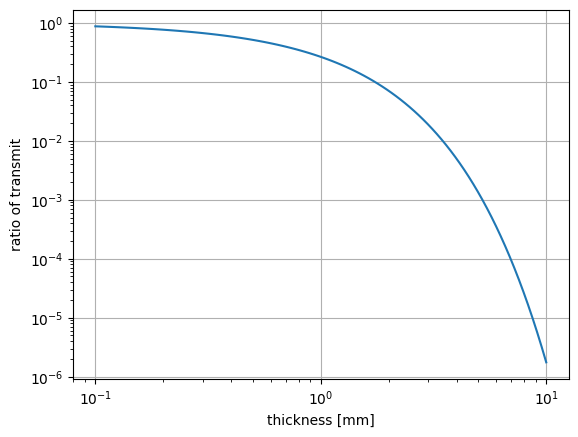
遮蔽の厚さに対する吸収率を図にする

import matplotlib.pyplot as plt
import numpy as np
x = np.logspace(-1, 1, 100, 'base=10') ## mm
y_val = -N_B4C*x*1e-3*(sigma_roi)*1e-28
y =np.exp(y_val)
plt.plot(x, y, label="trans")
plt.xlabel('thickness [mm]')
plt.ylabel('ratio of transmit')
plt.grid()
plt.xscale('log')
plt.yscale('log')
plt.show()

運動量移行の計算

運動量移行\(q\)はその波長\(\lambda\)、移動角\(\theta\)を用いて \[ q = 4\pi\frac{\sin\theta}{\lambda} \] と書ける。 ここで\(\theta\)とは、透過ビームと反射ビームの角度差の1/2であることに留意。

#final update
!echo final update
!date '+%b %d %Y (%a)'

final update
 8月 10 2026 (月)